图像压缩原理及 libjpeg 源码分析
最近在做图像处理项目的性能优化时发现,RGB 转 JPG 压缩的文件大小有波动,而这个会显著影响图像上传耗时。
为什么会有波动呢?通过了解 JPG 压缩编码的原理,我找到了答案。
为何数据能压缩
频域编码
相信大家对哈夫曼编码不陌生,它根据字符出现频率编码:频率越高,编码越长。其实就是利用频域编码压缩文本。
同样,图像也具有频域特性:由于视觉暂留,人眼对高频信息不敏感:
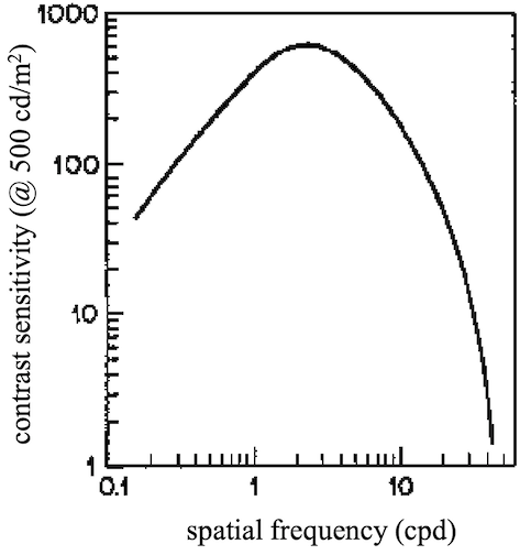
One reason why the eye has reduced sensitivity at high frequencies is because it can retain the sensation of an image for a short interval after the image has been removed, a phenomenon known as persistence of vision.
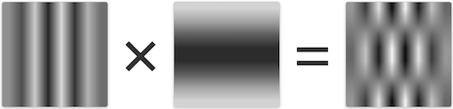
如果对于上面的图和描述云里雾里,可以通过下面这张图来直观地感受下:
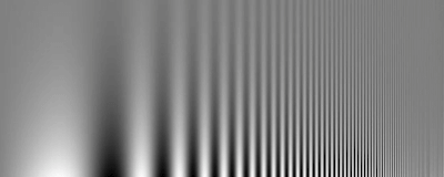
从左往右,条纹明暗变化频率变快,肉眼越来越难辨别。
所以我们可以过滤掉高频部分,达到压缩图像的目的。
频域变换
如何将图像转为频域信息呢?
学过数字信号处理的一定对傅里叶变换不陌生,不太熟悉的可以看 Eugene Khutoryansky 的视频。
这里不做公式推导,简单说就是:任何信号可以转换为一系列特定频率波的叠加。
上图演示了方波信号的合成,更多有趣的合成效果可以移步 An Interactive Introduction to Fourier Transforms。
傅里叶变换最初主要用于通信领域,一般约定俗成的说法是:将 时域信号 转换为 频域信号。
而在图像处理领域,时域信号实际指的是 像素的空间分布。
从更广泛的数学意义上来说,本质是通过正交基变换,将数据映射到一组更容易分析处理的空间维度上。
频域分析之所以普适,是因为以声音/图像为代表的物理信号天然适合频率描述和处理:人的感官对高频明暗和声音变化不敏感。
由于图像数据是离散的、有限长的,且只有实数部分(傅里叶变换是复数域的),所以实际用的更多的是离散余弦变换。
下面我们详细看下 JPG 压缩过程。
JPG 压缩编码过程
YUV 降采样
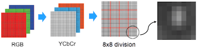
首先第一步是 RGB 转 YUV。
通过前文可知:人眼对明暗和绿色更敏感,YUV420 相当于降采样,相比 RGB 数据量更少。
所以这一步转换既减少了后续处理的数据量,同时也相当于做了部分压缩(丢掉了不敏感信息)。
数据分块
并且为了后续处理方便,将 YUV 每个通道分为一个个区块(通常是 8x8):
区间映射
假设原来 block 的矩阵为:
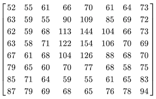
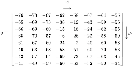
为了减少绝对值的波动,将其从 [0, 255] 映射到关于 0 对称的 [-128, 127]:
离散余弦变换
有一个 8x8 的基底余弦波:
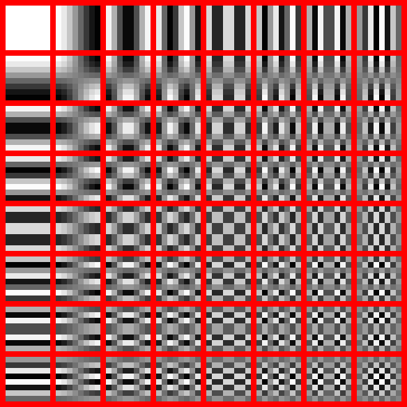
从左往右/从上往下频率变高;最左上角那个是直流(DC)分量,其余 63 个是交流(AC)分量。
这个 8x8 的图怎么来的呢?其实就是不同频率水平和竖直方向明暗条纹的叠加:
通过这些余弦波的系数来表示原来的图像:
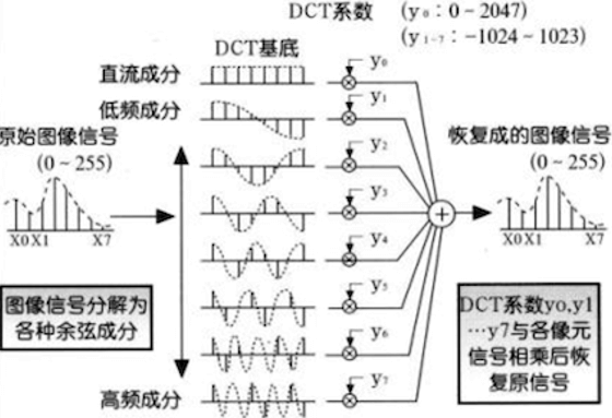
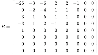
余弦变换后得到如下的矩阵:
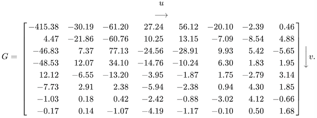
至此,原始的图像已经转化为频域数据(跟基底矩阵一样,右下角也是高频部分)。
需要注意的是:这一步还是无损的。
量化
量化就是拿频域数据逐项除以一个量化矩阵的值并取整。
为什么要这么操作呢?
前面我们提到,人眼对高频明暗变化不敏感,因此这个量化矩阵右下角高频区数值较大,量化后更容易得到 0(可以舍弃),这样就能过滤掉人眼不敏感的高频数据。
比如压缩质量为 50 对应的量化矩阵为:
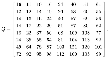
然后将两个矩阵逐项相除并取整。量化后得到的矩阵为:
显然,这一步是有损的。
熵编码
由于相邻图块之间的 DC 系数(最左上角)间一般有很强的相关性,所以对 DC 系数采用 DPCM 编码,即对相邻像素块之间的系数差值进行编码。
其余 63 个交流分量 AC 系数如下的游程编码:
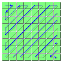
这种扫描方式可以将频率相近的编码在一起,以得到更多的 0:
−26
−3	0
−3	−2	−6
2	−4	1	−3
1	1	5	1	2
−1	1	−1	2	0	0
0	0	0	−1	−1	0	0
0	0	0	0	0	0	0	0
0	0	0	0	0	0	0
0	0	0	0	0	0
0	0	0	0	0
0	0	0	0
0	0	0
0	0
0
连续的 0 就可以进一步压缩编码为:
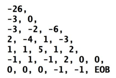
这里实际上也用到了前面提到的哈夫曼编码,可谓殊途同归:最终还是变成了文本压缩。
libjpeg 源码分析
Talk is cheap. Show me the code!
下面我们结合 libjpeg-turbo 源码来看看图像压缩过程。
离散余弦变换
大家可能见过世面上各种魔改 Android 自带的 JPG 压缩,号称是提升了性能或质量;乍一看很牛,其实主要就是调整余弦变换的参数。
具体就是 jpeg_compress_struct 里面有个 dct_method 成员:
struct jpeg_compress_struct {
    ...
    J_DCT_METHOD dct_method;      /* DCT algorithm selector */
    ...
}
定义为:
typedef enum {
  JDCT_ISLOW,             /* accurate integer method */
  JDCT_IFAST,             /* less accurate integer method [legacy feature] */
  JDCT_FLOAT              /* floating-point method [legacy feature] */
} J_DCT_METHOD;
其实主要就是 JDCT_IFAST 或者 JDCT_ISLOW。
通过查阅官方文档可知:
在 X86 设备上,二者性能相差不大,在其他设备上,前者比后者快 5-15%;
当 quality 低于 90 时,二者的质量相差不大;
当 quality 高于 97 时,
JDCT_IFAST不仅没有被完全加速(性能更低),而且质量也显著降低;
所以我们可以根据压缩质量去动态选择变换算法,或者根据实际场景(是更关注时间还是质量)去选择。
量化表
JQUANT_TBL 定义了量化表数据结构:
typedef struct {
  /* This array gives the coefficient quantizers in natural array order
   * (not the zigzag order in which they are stored in a JPEG DQT marker).
   * CAUTION: IJG versions prior to v6a kept this array in zigzag order.
   */
  UINT16 quantval[DCTSIZE2];    /* quantization step for each coefficient */
  /* This field is used only during compression.  It's initialized FALSE when
   * the table is created, and set TRUE when it's been output to the file.
   * You could suppress output of a table by setting this to TRUE.
   * (See jpeg_suppress_tables for an example.)
   */
  boolean sent_table;           /* TRUE when table has been output */
} JQUANT_TBL;quantval[]数组就是量化表数据;sent_table这个标志位用来标识量化表是否已经被写入到 JPG 文件。
而压缩信息 jpeg_compress_struct 包含一个量化表数组成员:
struct jpeg_compress_struct {
    ...
    JQUANT_TBL *quant_tbl_ptrs[NUM_QUANT_TBLS];
#if JPEG_LIB_VERSION >= 70
  int q_scale_factor[NUM_QUANT_TBLS];
#endif
  /* ptrs to coefficient quantization tables, or NULL if not defined,
   * and corresponding scale factors (percentage, initialized 100).
   */
   ...
}
设置压缩质量
先看 jpeg_set_quality() 函数:
GLOBAL(void)
jpeg_set_quality(j_compress_ptr cinfo, int quality, boolean force_baseline)
/* Set or change the 'quality' (quantization) setting, using default tables.
 * This is the standard quality-adjusting entry point for typical user
 * interfaces; only those who want detailed control over quantization tables
 * would use the preceding three routines directly.
 */
{
  /* Convert user 0-100 rating to percentage scaling */
  quality = jpeg_quality_scaling(quality);

  /* Set up standard quality tables */
  jpeg_set_linear_quality(cinfo, quality, force_baseline);
}
先对 quality 做范围调整,然后调用 jpeg_set_linear_quality():
GLOBAL(void)
jpeg_set_linear_quality(j_compress_ptr cinfo, int scale_factor,
                        boolean force_baseline)
/* Set or change the 'quality' (quantization) setting, using default tables
 * and a straight percentage-scaling quality scale.  In most cases it's better
 * to use jpeg_set_quality (below); this entry point is provided for
 * applications that insist on a linear percentage scaling.
 */
{
  /* Set up two quantization tables using the specified scaling */
  jpeg_add_quant_table(cinfo, 0, std_luminance_quant_tbl, scale_factor, force_baseline);
  jpeg_add_quant_table(cinfo, 1, std_chrominance_quant_tbl, scale_factor, force_baseline);
}
注意这里第三个参数传的是两个标准量化表:
/* These are the sample quantization tables given in Annex K (Clause K.1) of
 * Recommendation ITU-T T.81 (1992) | ISO/IEC 10918-1:1994.
 * The spec says that the values given produce "good" quality, and
 * when divided by 2, "very good" quality.
 */
static const unsigned int std_luminance_quant_tbl[DCTSIZE2] = {
  16,  11,  10,  16,  24,  40,  51,  61,
  12,  12,  14,  19,  26,  58,  60,  55,
  14,  13,  16,  24,  40,  57,  69,  56,
  14,  17,  22,  29,  51,  87,  80,  62,
  18,  22,  37,  56,  68, 109, 103,  77,
  24,  35,  55,  64,  81, 104, 113,  92,
  49,  64,  78,  87, 103, 121, 120, 101,
  72,  92,  95,  98, 112, 100, 103,  99
};
static const unsigned int std_chrominance_quant_tbl[DCTSIZE2] = {
  17,  18,  24,  47,  99,  99,  99,  99,
  18,  21,  26,  66,  99,  99,  99,  99,
  24,  26,  56,  99,  99,  99,  99,  99,
  47,  66,  99,  99,  99,  99,  99,  99,
  99,  99,  99,  99,  99,  99,  99,  99,
  99,  99,  99,  99,  99,  99,  99,  99,
  99,  99,  99,  99,  99,  99,  99,  99,
  99,  99,  99,  99,  99,  99,  99,  99
};
std_luminance_quant_tbl 用于亮度(Y 通道),std_chrominance_quant_tbl 用于色度(UV 通道)。
最终调用的是 jpeg_add_quant_table():
GLOBAL(void)
jpeg_add_quant_table(j_compress_ptr cinfo, int which_tbl,
                     const unsigned int *basic_table, int scale_factor,
                     boolean force_baseline)
/* Define a quantization table equal to the basic_table times
 * a scale factor (given as a percentage).
 * If force_baseline is TRUE, the computed quantization table entries
 * are limited to 1..255 for JPEG baseline compatibility.
 */
{
  JQUANT_TBL **qtblptr;
  //...
  if (*qtblptr == NULL)
    *qtblptr = jpeg_alloc_quant_table((j_common_ptr)cinfo);
  for (i = 0; i < DCTSIZE2; i++) {
    temp = ((long)basic_table[i] * scale_factor + 50L) / 100L;
    /* limit the values to the valid range */
    if (temp <= 0L) temp = 1L;
    if (temp > 32767L) temp = 32767L; /* max quantizer needed for 12 bits */
    if (force_baseline && temp > 255L)
      temp = 255L;              /* limit to baseline range if requested */
    (*qtblptr)->quantval[i] = (UINT16)temp;
  }
  //...
}
首先初始化量化表数组
qtblptr;然后将基准量化表
basic_table每一项乘以压缩系数scale_factor,得到新的量化表,并添加到量化表数组;最后将
qtblptr的sent_table置为FALSE,最终新的量化表数组会被写入 JPG 文件。
可以看到,这里实际上只是将标准量化表乘了一个系数 scale_factor,而前面他是直接将 quality 传过来的。
不知道大家发现问题没有:
前面我们提到,量化就是将频域数据逐项除以量化表再取整,量化表值越大,越容易得到 0 从而压缩数据,因此右下角高频区数值相对更大。
但是,这里直接拿 quality 乘以量化矩阵,质量越大量化矩阵值越大,最后数据越失真,岂不是前后矛盾?
原来前面还调用了 jpeg_quality_scaling():
GLOBAL(int)
jpeg_quality_scaling (int quality)
/* Convert a user-specified quality rating to a percentage scaling factor
 * for an underlying quantization table, using our recommended scaling curve.
 * The input 'quality' factor should be 0 (terrible) to 100 (very good).
 */
{
  /* Safety limit on quality factor.  Convert 0 to 1 to avoid zero divide. */
  if (quality <= 0) quality = 1;
  if (quality > 100) quality = 100;

  /* The basic table is used as-is (scaling 100) for a quality of 50.
   * Qualities 50..100 are converted to scaling percentage 200 - 2*Q;
   * note that at Q=100 the scaling is 0, which will cause jpeg_add_quant_table
   * to make all the table entries 1 (hence, minimum quantization loss).
   * Qualities 1..50 are converted to scaling percentage 5000/Q.
   */
  if (quality < 50)
    quality = 5000 / quality;
  else
    quality = 200 - quality*2;

  return quality;
}
这里利用反函数,巧妙地将用户层面的图像质量映射到代码实现层面的矩阵采样系数。这样就能说得通了。
哈夫曼编码
首先有个哈夫曼表的数据结构定义,类似量化表:
typedef struct {
  /* These two fields directly represent the contents of a JPEG DHT marker */
  UINT8 bits[17];               /* bits[k] = # of symbols with codes of */
                                /* length k bits; bits[0] is unused */
  UINT8 huffval[256];           /* The symbols, in order of incr code length */
  /* This field is used only during compression.  It's initialized FALSE when
   * the table is created, and set TRUE when it's been output to the file.
   * You could suppress output of a table by setting this to TRUE.
   * (See jpeg_suppress_tables for an example.)
   */
  boolean sent_table;           /* TRUE when table has been output */
} JHUFF_TBL;同样,jpeg_compress_struct 也包含两个哈夫曼表数组成员:
struct jpeg_compress_struct {
    ...
    JHUFF_TBL *dc_huff_tbl_ptrs[NUM_HUFF_TBLS];
    JHUFF_TBL *ac_huff_tbl_ptrs[NUM_HUFF_TBLS];
    /* ptrs to Huffman coding tables, or NULL if not defined */
   ...
}
dc_huff_tbl_ptrs 用于对左上角直流(DC)部分作差分编码,ac_huff_tbl_ptrs 用于对剩余交流(AC)部分作游程编码。
视频编码中的图像压缩
由于视频每一帧也是 YUV,所以视频压缩编码的核心流程跟上面的 JPG 压缩是一致的:
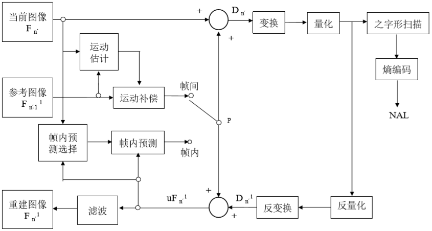
只不过在最前面加了一步帧预测,去除时域的冗余信息:通过先前的图像来预测和补偿当前的局部图像。
其实早期的 H.261 就是直接基于离散余弦变换,而后续的 H.264、H.265 也都用到了离散余弦变换、量化、熵编码等图像压缩核心技术。
关于文件大小
文件大小波动的原因
我们再回头看看开头的问题:为什么 JPG 压缩后的文件大小会有波动呢?
从前文可知:数据量减小的关键,就是通过量化将不敏感的高频部分尽量变成 0,从而通过熵编码过滤掉。
所以我这里大胆猜测,输出的 JPG 文件大小波动可能是因为:
每一帧的像素分布不同,产生的频域矩阵不同,最后量化后得到的 0 数量也不同。
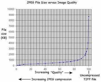
文件大小跟压缩质量的关系
从前文余弦变换参数可知:90 是压缩质量的一个坎,高于 90 时,不同算法对性能和质量的影响差异明显。
日常使用中,我们也一般将压缩质量设置为 90;因为高于 90 后,输出文件大小会指数级增长: